Sudoku Variants

Most are familiar with the 9x9 Sudoku grid often found in the back of any newspaper. The rules are simple: each row, column, and 3x3 region must uniquely contain the values 1 through 9, and there can be only one solution for the initial values given. These rules alone can produce some very interesting and difficult puzzles, but the traditional rules can be further expanded to produce some interesting and unique challenges as well. Common variations either change the size of the board, the shape of the the sub-regions (where 3x3 squares are normally used), or impose additional constraints on what values a cell can take. The particular puzzle which inspired this article is the 'Magic Square Sudoku' by Aad van de Wetering which adds a few interesting constraints to make an otherwise unsolvable puzzle, solvable.

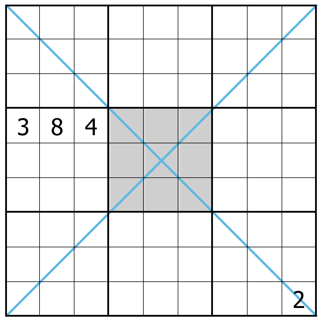
A Sudoku with only 4 digits given could never have a single unique solution; in fact, the minimum is 17. Therefore, in order for this puzzle to be solvable it's creator has imposed three constraints in addition to the standard rules.

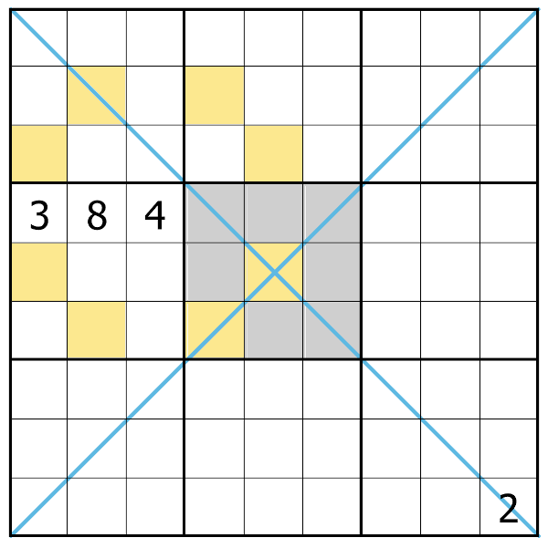
The first additional constraint is that values along the two diagonal axis (marked with blue lines in the image) also uniquely contain the values 1 through 9. The second rule states that the center 3x3 square is also a Magic Square. This means the values of it's rows, columns, and diagonals all sum to the same value. The final additional rule is known as an 'anti-knight' constraint, in reference to the movements of the knight in chess. This rule states cells which are a knight's move apart cannot contain the same value. In the example below, cells coloured yellow cannot also contain the value 4 due to this constraint.

An Optimization Problem

If you'd like to see this puzzle solved by hand, YouTuber CrackingTheCryptic has a great video walking through it step-by-step. Instead, I'll be using linear programming to solve this problem. Linear Programming is a method to optimize a linear objective function given a system of linear constraints. Sudoku can be expressed as a specific type of linear program knows as a binary integer linear program.

Posing a Sudoku as a linear program is not a new idea; thorough examples do a great job of explaining every step of translating the Sudoku puzzle to a set of linear constraints. In brief summary, for every cell we introduce 9 binary decision variables, for a total of 729 to represent the puzzle. Each decision variable - indexed by it's row, column, and value - reflects whether or not that value is picked for that cell. For example if X₁₁₃ = 1, this means that the value of the cell in the top left corner is 3. You will also notice we use an arbitrary constant objective function, as there is no way to improve a Sudoku solution we are just looking for a set of values which satisfies all the constraints. With that, here is the linear program for the standard Sudoku rules:

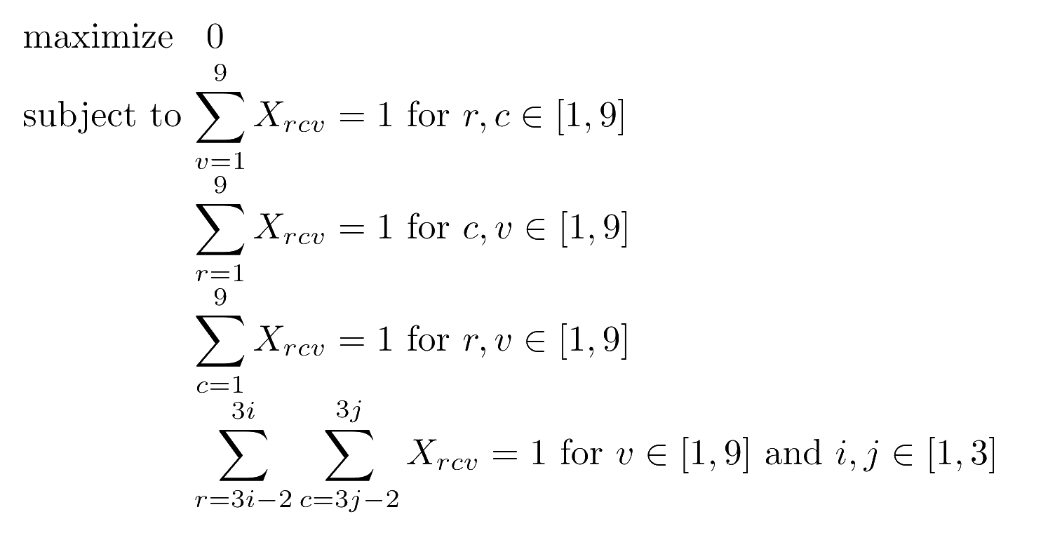
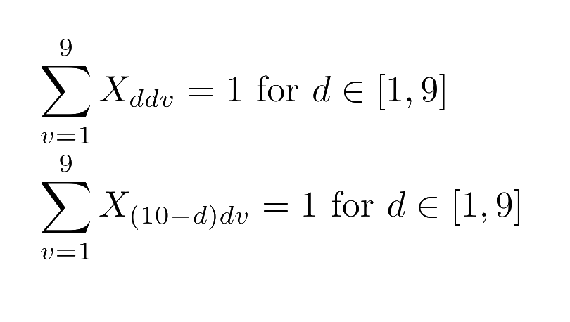
The first sum constrains each cell, indexed by it's row and column to take on only one value. The next two constraints reflect the standard rule that each row and column contain the values 1 through 9 uniquely. The fourth sum maintains that each sub-grid also contains the values 1 through 9. In order to incorporate the additional rules of the Magic Square Sudoku we'll need a few more constraints. The first two additional summations express that along each diagonal, the values between 1 and 9 appears exactly once.

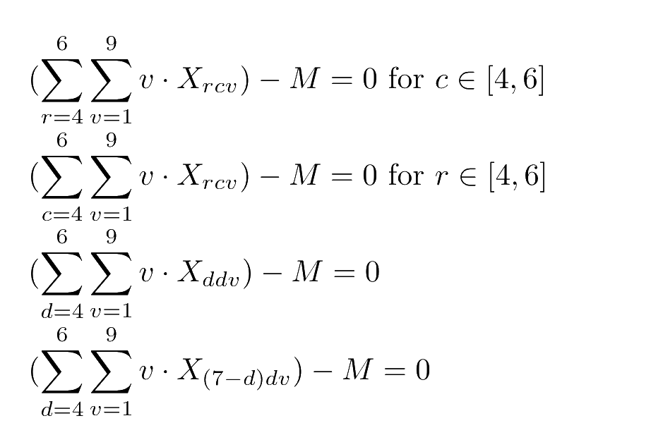
To pose the magic square constraint as a linear expression we need to introduce a single additional decision variable M. The value of this variable is the magic number for the magic square, which each row, column, and diagonal sum to. The nuance of these equations is in multiplying the variable index v by the value of X_rcv which is either a binary 1 or 0 to get the real value of the cell. We sum these values along each row, column, and diagonal of the center 3x3 grid, then subtract M to enforce that everything equals the same value.

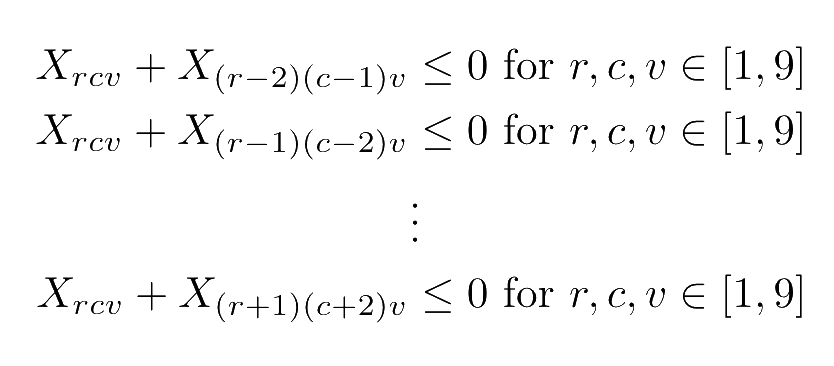
Translating the knight's move constraint to a system of linear expressions is a bit more challenging. Intuitively, it would be nice to use the same trick from our magic square constraint to get the actual value of a cell, then compare it to that of the cells in the knight's move positions. Unfortunately, the idea of 'not equals' is harder to encode; it can be done by introducing an additional boolean variable but there's an easier way to represent this constraint for our specific problem.

Instead of trying to encode the idea that 'the value of cell A is not equal to the value of cell B', we can enforce that 'at most one of cell A or cell B can have value X'. For each cell, we iterate over every value and check that either one or zero of those cells has that value set. This achieves the effect we want, but it comes at a cost of adding 9 inequalities for every knights move of every cell on the board. In a theoretical context this doesn't matter, but we'll see when we actually build a solver that this has a real impact on the time to find a solution. There are a few optimizations which can reduce the actual number of knight's move positions considered but overall they still make up over 90% of the constraints in the model.

Solving the Puzzle

I'll be using the Python linear programming library PuLP to handle the heavy lifting of actually solving linear programs. Instead of writing a Sudoku solver from scratch I'll be building on top of PuLP's own implementation of a generic Sudoku solver. I'll focus on the code for the new constraints I've added in this article, but the full source code can be found on my Github here.

Diagonals

Translating the constraints for the diagonals from their mathematical expressions to Python code is almost identical to the existing constraints for the rows and columns. PuLP's lpSum calculates a sum from a vector of linear expressions. We can then add this as a constraint directly to our problem.

# Each major diagonal contains only one of each value
for v in VALS:
    prob += lpSum([choices[d][d][v] for d in DIAGONAL]) == 1
    prob += lpSum([choices[10 - d][d][v] for d in DIAGONAL]) == 1

Magic Square

The magic square constraint follows a similar pattern. Similarly to the diagonal constraints, this is a pretty faithful recreation of the mathematical expression we defined earlier so there's not a lot of surprises.

# The sum of each row, column and diagonal of the magic square is the same
for r in range(3):
    prob += lpSum([v * choices[4 + r][4 + c][v] for v in VALS for c in range(3)] + (magic_square * -1)) == 0

for c in range(3):
    prob += lpSum([v * choices[4 + r][4 + c][v] for v in VALS for r in range(3)] + (magic_square * -1)) == 0

prob += lpSum([v * choices[4 + d][4 + d][v] for d in range(3) for v in VALS] + (magic_square * -1)) == 0
prob += lpSum([v * choices[6 - d][4 + d][v] for d in range(3) for v in VALS] + (magic_square * -1)) == 0

In linear programming, we want our decision variables on the left side of the expression. This is how I've expressed it in the mathematical equation as well as the code but PuLP is pretty flexible and could just as easily handle a statement of the following form

prob += lpSum([v * choices[6 - d][4 + d][v] for d in range(3) for v in VALS]) == magic_square

We can take a peek under the hood of PuLP by looking at the MagicSquare.lp file our code generates (it's a plaintext file, you can open it in any text editor) to see how these equations are handled.

_C350: choice_4_6_1 + 2 choice_4_6_2 + 3 choice_4_6_3 + 4 choice_4_6_4
 + 5 choice_4_6_5 + 6 choice_4_6_6 + 7 choice_4_6_7 + 8 choice_4_6_8
 + 9 choice_4_6_9 + choice_5_5_1 + 2 choice_5_5_2 + 3 choice_5_5_3
 + 4 choice_5_5_4 + 5 choice_5_5_5 + 6 choice_5_5_6 + 7 choice_5_5_7
 + 8 choice_5_5_8 + 9 choice_5_5_9 + choice_6_4_1 + 2 choice_6_4_2
 + 3 choice_6_4_3 + 4 choice_6_4_4 + 5 choice_6_4_5 + 6 choice_6_4_6
 + 7 choice_6_4_7 + 8 choice_6_4_8 + 9 choice_6_4_9 - magic_square_sum = 0

This is a line from the LP which correlates to a single expression from the magic square. As we see even though it was generated with magic_square_sum on the right of the equation PuLP has rewritten the expression with it on the left. Trés neat!

Knight's Move

For the knight's move we define the eight possible knight's move offsets as a constant. We iterate over every cell and define a constraint for every value expressing that either one or fewer of the cells can take that value. As mentioned before, the knight's move constraint generates most of the complexity of our model. I've add a variable outside of the linear program to keep track of the number of constraints we generate here. With no optimizations, that number is 4032 out of 4386 total constraints in the model.

To reduce this I've included a simple optimization in the helper function to protect against invalid indices. It also ignores the constraint if the knight's move falls within the same 3x3 grid that the target cell is in. This works because that case is trivially covered by the standard Sudoku rules for 3x3 sub-grids. This simple check reduces the total number of constraints in our model to 3090, with 2736 being from knight's moves.

# Each of the valid knights moves
KNIGHTS_MOVES = [(-1, -2), (-2, -1), (-2, 1), (-1, 2), (1, 2), (2, 1), (2, -1), (1, -2)]
knights_move_constraint_count = 0

# Helper function to avoid invalid indices as well as a small optimization to avoid checking knight's moves
# in the same 3x3 square
def isUsefulKnightsMove(r, c, r_off, c_off):
    r_tgt = r + r_off
    c_tgt = c + c_off

    return (1 <= r_tgt <= 9
        and 1 <= c_tgt <= 9
        and (math.ceil(r / 3) != math.ceil(r_tgt / 3) or math.ceil(c / 3) != math.ceil(c_tgt / 3 )))

# Create the knight's moves constraints
for r in ROWS:
    for c in COLS:
        for (r_off, c_off) in KNIGHTS_MOVES:
            if isUsefulKnightsMove(r, c, r_off, c_off):
                for v in VALS:
                    expr = [choices[r][c][v], choices[r + r_off][c + c_off][v]]
                    prob += lpSum(expr) <= 1
                    knights_move_constraint_count += 1

Exploring ways to further optimize this problem would be a worthwhile exercise. For starters you could significantly reduce the number of constraints by considering the fact that if cell A is a knight's move from cell B, cell B is also a knight's move from cell A. In other words, every knight's move constraint is duplicated by the paired cell. My understanding is part of the pre-processor for the generic PuLP solver tries to eliminate as many trivially redundant constraints as it can so whether this will really make a difference is questionable but at the very least you can reduce the size of the model.

Solution

If you've followed along - or just cloned the code - that's all the pieces. You can finally complete the puzzle and solve the Magic Square Sudoku. Running the script may take a couple minutes to solve the linear program, but once it's finished it will write the result to a file. The snippet below shows how you can run the program from your terminal and view the output.

$ python3 sudoku.py
$ cat sudokuout.txt
+-------+-------+-------+
| 8 4 3 | 5 6 7 | 2 1 9 |
| 2 7 5 | 9 1 3 | 8 4 6 |
| 6 1 9 | 4 2 8 | 3 7 5 |
+-------+-------+-------+
| 3 8 4 | 6 7 2 | 9 5 1 |
| 7 2 6 | 1 5 9 | 4 8 3 |
| 9 5 1 | 8 3 4 | 6 2 7 |
+-------+-------+-------+
| 5 3 7 | 2 8 6 | 1 9 4 |
| 4 6 2 | 7 9 1 | 5 3 8 |
| 1 9 8 | 3 4 5 | 7 6 2 |
+-------+-------+-------+

Magic Square Sum: 15.0
Knights Move Constraints: 2736
Total Constraints: 3090

Trevor McCann • November 2020